Fundamentals – GM Hydro

General

Hydraulic turbines belong to the category of motor driven machines and can be classified following various criteria, nevertheless the most used one concerns the type of energy transformation they carry out. Then, we distinguish the turbines in IMPULSE turbines and REACTION turbines. The first category includes PELTON turbines (fig 1) where the potential energy , E_p = mgH (m=mass, g= gravity acceleration, H= head) is transformed into kinetic energy ${ E }_{ c }=\frac { 1 }{ 2 } m{ v }^{ 2 }$ with v= velocity of the fluid before acting on the runner buckets. This means that the fluid strikes the runner with a velocity corresponding to about $v\cong\sqrt { 2gH }$

fig 1

fig 2

fig 3

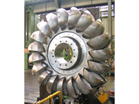
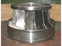
FRANCIS (fig 2) and KAPLAN turbines (fig 3) are of the REACTION type. Their respective runners have the task to transform into kinetic energy the remaining potential energy still available.

Pelton Runner

Francis Runner

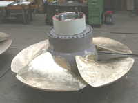
Kaplan Runner

This category includes also the BULB turbines (fig 4) and the S turbines (fig 5) .

fig 4

fig 5

The first two main quantities necessary for the dimensioning of one hydraulic turbine are:
1) H = available net head [m] 2) Q = discharge of the fluid [m³/s]

fig 6 – net head quote (A) impulse turbines (B) reaction turbines

Said $\gamma$ the fluid specific weight, the turbine efficiency, the power generated by the turbine expressed in Kw will be:
P= $\bf\frac {{\large \gamma} QH{\large \eta }}{ 101,97 }$ assumed for the water $\gamma$ = 1000 Kg/m³P ≈ 9,81 Q H η [a]
The same expression may be used to calculate the power of the generating unit but in this case the efficiency $\eta$ of the turbine has to be replaced with the total one ${\eta}_{t}$ obtained by the product of the efficiencies of each single component (turbine, generator, transformer). Finally, from the obtained power it will be necessary to subtract the one pertaining to the mechanical losses (for example those concerning the bearings) and the volumetric losses (for example those concerning the discharge of the water under pressure between cover and runner)

Specific rotation speed
Suppose we have a turbine operating with H, Q, n and that we want to operate with the same runner with head H’ different from H. The new absolute speed shall beand e v’= $\sqrt { 2gH }$ then we can write: $\frac {\large v }{\large v' } =\frac { \sqrt { 2gH} }{ \sqrt { 2gH'}} =\sqrt {\frac { H}{ H'} }$
In the here figures shown below, the symbol 1 indicates the speeds at the runner inlet whereas 2 indicates the runner outlet ones.

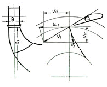
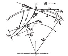
We are talking about peripheral u, absolute v and relative w speeds. In order that everything may operate regularly, it is necessary to have the equality: $\frac {\large v }{\large v' } =\frac {\large u}{\large u'}=\frac {\large w}{\large w'} =\sqrt { \frac { H}{ H'} }$
Since the runner has not been changed, also the flow through the interblade channel will vary in accordance with the new speed w’. As a consequence we can write : $\frac {\large w }{\large w' } =\frac { Q}{ Q'} =\sqrt { \frac { H}{ H'} }$
The peripheral speed u is connected to the rotation speed and, likewise, we can write : $\frac {\large u }{\large u' } =\frac {\large n}{\large n'} =\sqrt {\frac { H}{ H'} }$

In conclusion of what said above, we can state that the runner operating with H, Q, n can operate correctly also with H’, Q’, n’
Again, what said above allows us to make another important consideration. The same runner, instead of operating under the head H, will operate under the head of 1 m. Applying the same above described relations and indicating with the subscript 1 the values relevant to the new conditions, we can write:
$\frac { Q}{{ Q}_{1}} =\sqrt { \frac { H}{ 1} }$       Q₁= $\bf\frac { Q}{ \sqrt { H}}$                $\frac {\large n}{{\large n}_{1}} =\sqrt { \frac { H}{ 1} }$                    n₁= $\bf\frac {\large n}{ \sqrt { H}}$
Now we see how the previous relations allow us to write those relevant to the change of runner diameter passing from the value D to the value of 1 m. All geometrical dimensions of the runner will vary in the same ratio until to obtain the diameter of 1 m. We know that the head is H = 1 m and then the absolute speed at the inlet of the new runner shall be the same with respect to that of diameter C. This allows to state that also the other speeds will remain unchanged because they are connected one another by the triangle of speeds (see above figure).

We have seen that the speeds have not changed, therefore the flow discharged by the new runner will inevitably vary following the same variation ratio of the respective sections of the water passage and hence also in accordance with the respective diameters. Said the new discharge, we can write:
$\frac { { Q}_{11}}{{ Q}_{1}} =\frac { { 1}^{2}}{{ D}^{2}}$                 Q₁₁= $\frac { { Q}_{1}}{{ D}^{2}}$                       Q₁₁= $\bf\frac { { Q}_{1}}{{ D}^{2}\sqrt { H}}$
We passed from diameter D to the diameter of 1 m and since the speeds are the same for both runners, in particular the peripheral one, the rotation speed will be inevitably modified.
$\frac { {\large n}_{11}}{{\large n}_{1}} =\frac { D}{ 1}$                 n₁₁=n₁D                       n₁₁= $\bf\frac {{\large n}D}{\sqrt { H}}$
are defined respectively specific rotation and specific flow.
They therefore represent the number of revolutions and the flow that one runner having diameter D=1m and H=1m has to operate in order to keep unchanged the initial operating conditions of a similar runner with diameter D and head H.

Example
We have one turbine operating under the following rated data:
H = 130 m Q= 25 m³/s   n= 500 rpm and runner diameter D = 1,68 m
From previous relations, we obtain:
Q₁₁= 0,777    n₁₁= 73,673
The same runner may be used with the new values of H, Q, n if Q₁₁ e n₁₁ remain unchanged
For example with H= 95 m   Q= 21,4 m³/s we obtain n=427 rpm

Characteristic speed
UOne of the most used expressions to classify one runner is the one that allows calculating its “Characteristic Number of Revolutions”. This represents the speed n in rpm of one runner similar to the one that is considered under the head of H = 1 m and the discharge Q=1 m³/s. This number is expressed as : n_q=n $\bf \frac {\sqrt{Q}}{ { H }_{ }^{ 0,75 } }$ [b]
A first classification can be made in accordance with the following table :

nq = 6 ÷ 20	slow speed machines	Pelton
nq = 20 ÷ 100	average speed machines	Francis
nq > 100	fast speed machines	Kaplan

Note.
The classification slow, average, fast is not connected to the operating speed but to the value of nq. With high nq values, in general we have low operating speed (Kaplan).

With the data of the previous example we obtain: n_q=500 $\frac {\sqrt {25}}{ { 130 }_{ }^{ 0,75 }}$ ≈ 65

We see how the expression of nq is obtained.
Given one turbine operating with H-Q-n and with runner having diameter D. We feed the same runner with H=1 m (we obtain Q₁ and n₁) and then with Q_c=1 m³/s . If we use the previous relations, we can write:
$\frac { { Q}_{1}}{{ Q}_{c}} =\frac { { D}^{2}}{{ D}_{c}^{2}}$ $\frac { D}{{ D}_{c}}=\sqrt\frac { { Q}_{1}}{{ Q}_{c}}$ $\frac{ D}{{ D}_{c}}=\sqrt{\frac {{Q}_{1}}{1}}$ $\frac { D}{{ D}_{c}}=\sqrt{{\scriptsize Q}_{\scriptsize 1}}$
Likewise
$\frac { {\large n}_{c}}{{\large n}_{1}} =\frac { D}{{ D}_{c}}$ ${ n}_{c}={n}_{\scriptsize 1}\sqrt {\scriptsize Q}_{\scriptsize 1}$ ${ n}_{c}=\frac {\large n}{\sqrt { H}}\sqrt{\frac { Q}{\sqrt { H}}}$

to fix n_c=n_q we have: n_q=n $\bf \frac { \sqrt{ Q}}{ { H }_{ }^{ 0,75 } }$
The hydraulic turbines manufacturers have at their disposal for a reasonable series of nq one or more models tested in the laboratory. On the basis of the design data, it will be possible to calculate nq quickly, and then the nearest at disposal shall be selected. At this point, the hydraulic profile of the industrial machine (also called prototype) shall be obtained multiplying the geometrical data of the model by the ratio K=Dp/Dm (Dp = prototype runner diameter and Dm = model runner diameter).
The laboratory tests have the main purpose to determine the efficiencies the turbine can supply. This test campaign, besides several indications about the behavior of the turbine, gives the possibility to draw a diagram called “hill diagram” (see figure below) that depending on the values of H and Q, or of other quantities connected to them, allows to determine the turbine efficiency in that operating point. In general the prototype efficiency is higher than that obtained on model because for example the friction losses occurring inside the hydraulic passages have a lower influence. There are various step up formulas depending on the turbine type, but it is here not the case to describe calculations that go beyond the purpose of this site.

The model tests are an important inspection instrument for those who want to study new machines, but they are also very useful and important for the customers who whish to verify on a reduced scale, before the construction of the industrial turbine, its behavior in the future. One of the usual tests is the one that determines under which head and flow conditions the “torque”, that kind of tail made of bubbles originating under the runner, takes place. This phenomenon produces operating instability and power fluctuations more or less evident. The clips 1 and 2 show the “Torque” occurred in two different model tests of Francis turbine. It is important to verify that the torque takes place out of the normal operation zone. The torque is typical of the reaction machines and obviously doesn’t take place with the Pelton turbine.

As stated above, the coefficients that can be used for determining the axis of a hill diagram and/or identify the type of machine are several. The following table contains the most used ones.

n_q=n $\bf \frac { \sqrt{ Q}}{ { H }_{ }^{ 0,75 } }$

n_s=n $\bf\frac { \sqrt { P \bf\scriptsize (Kw) }}{ { H }_{ }^{ 1,25 } }$

n₁₁= $\bf\frac {{\large n}D}{\sqrt { H}}$

Q₁₁= $\bf\frac { Q}{{ D}^{2}\sqrt { H}}$

n_s= $\bf \scriptsize 3,1321\sqrt{\normalsize \eta}$ n_q

n_q= $\bf { n}_{\scriptsize 11}\sqrt {{\scriptsize Q}_{\scriptsize 11}}$

ns= $\bf\scriptsize 3,1321\sqrt{{\normalsize \eta}{ Q}_{11}}$ n₁₁

φ= $\bf\scriptsize 24,3171\frac{\normalsize Q}{{\normalsize D}^{\normalsize 3}\large n}$

ψ= $\bf\scriptsize 7153,60\frac{\normalsize H}{{\normalsize D}^{\normalsize 3}{\large n}^{\normalsize 2}}$

The following figures give an idea of the application fields of the various types of turbine

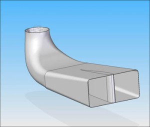
Draft Tube
When we deal with reaction turbines, we have to take into consideration one very important component, the Draft Tube. It has mainly the task to recovery the kinetic energy at the runner outlet into pressure energy, that is to recovery the head that on the contrary could be lost. This transformation becomes essential in turbines with low head, as for example Kaplan turbines, because the percentage of lost energy would be significant compared with the available head. Said the diameter of the tube just at the runner outlet, the velocity by which the water leaves the runner is v_s= $\bf\frac { 4Q }{{\large pi }{ D }_{\large s }^{ 2 } }$ (m/s) and the corresponding head that would be lost is H_p= $\bf\frac { {\large v }_{\large s }^{ 2 }}{\large 2g }$
A typical morphology is that represented in the following figure

Fig. 7 (gomito.jpg)